Genetic analysis of hereditary diseases with incomplete phenotypic manifestation / K. Eriksson.
- Eriksson, Karl, 1892-
- Date:
- 1954
Licence: Attribution-NonCommercial 4.0 International (CC BY-NC 4.0)
Credit: Genetic analysis of hereditary diseases with incomplete phenotypic manifestation / K. Eriksson. Source: Wellcome Collection.
54/64 page 52
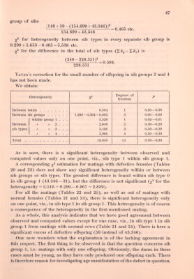
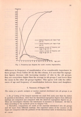
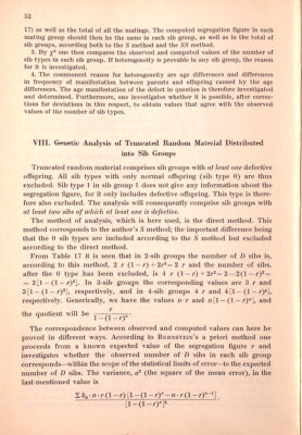
![52 17) as well as the total of all the matings. The computed segregation figure in each mating group should then be the same in each sib group, as well as in the total of sib groups, according both to the S method and the SS method. 3. By one then compares the observed and computed values of the number of sib types in each sib grouf). If heterogeneity is provable in any sib group, the reason for it is investigated. 4. The commonest reason for heterogeneity are age differences and differences in frequency of manifestation between parents and offspring caused by the age differences. The age manifestation of the defect in question is therefore investigated and determined. Furthermore, one investigates whether it is possible, after correc¬ tions for deviations in this respect, to obtain values that agree with the observed values of the number of sib types, VIII. Genetic Analysis of Truncated Random Material Distributed into Sib Groups Truncated random material comprises sib groups with at least one defective offspring. All sib types with only normal offspring (sib type 0) are thus excluded. Sib type 1 in sib group 1 does not give any information about the segregation figure, for it only includes defective offspring. This type is there¬ fore also excluded. The analysis will consequently comprise sib groups with at least two sibs of which at least one is defective. The method of analysis, which is here used, is the direct method. This method corresponds to the author's S method; the important difference being that the 0 sib types are included according to the S method but excluded according to the direct method. From Table 17 it is seen that in 2-sib groups the number of D sibs is, according to this method, 2 r (l — r^ + 2r^=2 r and the number of sibs, after the 0 type has been excluded, is 4 r (1 — r) + 2r^= 2^—2(1 —r)2 = = 2 [1 — (1 — ry]. In 3-sib groups the corresponding values are 3 r and 3[1 —(1 —r)®], respectively, and in 4-sib groups 4 г and 4[1 —(1 —r)^], respectively. Generically, we have the values n-r and л[1 —(1 —r)], and r the quotient will be -—^ • The correspondence between observed and computed values can here be proved in different ways. According to Bernstein's a priori method one proceeds from a known expected value of the segregation figure г and investigates whether the observed number of D sibs in each sib group corresponds—within the scope of the statistical limits of error—to the expected number of D sibs. The variance, (the square of the mean error), in the last-mentioned value is S/Tq-л-^(1 — r) [1 — (1 — r) —л •r(l — г) [l-(l-r)J](https://iiif.wellcomecollection.org/image/b18019754_0055.JP2/full/800%2C/0/default.jpg)