An investigation on the fate of organic and inorganic wastes discharged into the marine environment : and their effects on biological productivity.
- California. State Water Quality Control Board
- Date:
- 1965
Licence: Public Domain Mark
Credit: An investigation on the fate of organic and inorganic wastes discharged into the marine environment : and their effects on biological productivity. Source: Wellcome Collection.
34/134 page 20
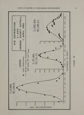
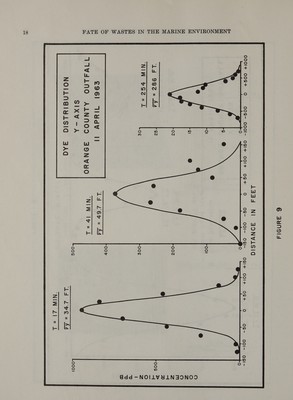
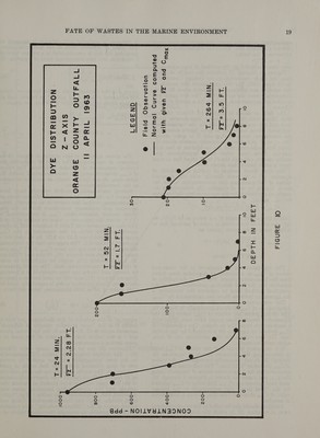
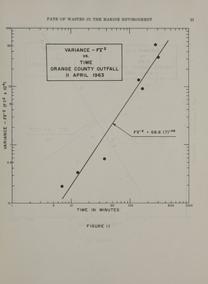
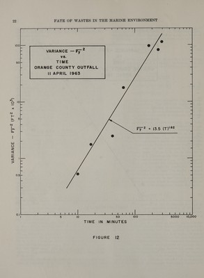
![defined a straight line. Empirical relationships for the variances of the form: o? == k(T)® (6) were then computed by the method of least-squares. Figures 11 through 13 indicate the results obtained from the study conducted at the Orange County site on 11 April 1963. For this experiment five pounds of dye solution was discharged at a point about 50 yards downstream from the surface boil. The dye patch was sampled at frequent time intervals for a period of about 6 hours. The data as shown in Figures 11, 12 and 13 have been fitted with the appropriate least-squares trend lines and the empirical equations for the variances are indicated. Visual inspection of these figures shows that the correlation between o*,,, and T is quite strong. The o?, vs. T plot shows considerable scatter about the trend line, indicating that the correlation is less sub- stantial. Data from other patch experiments give similar results, although the o?, vs. T trend line in most cases is much better than shown here. The most direct method of testing the validity of equation (1) is to work directly with the observed values of the maximum dye concentration within the patch, that is, by use of equation (2). Substituting the empirical expressions for the variances into the equation for Cmax yields: Cimax = 0.037 (T)-1-*! (Ib/ft?) Taking the specific weight of sea water as 64 lb/ft, we can also express the results in units of parts of dye to million parts of sea water (ppm) as: 0.037 = ——— 6 SUN Cmax 64 x 106(T) = 578(T)~'-*!(ppm) This expression can be compared to the measured values of Cmax as a function of dispersion time taken from the fluorometer record. The test of the validity of equation (2), the field sampling procedure, and of the analytical method used to compute the variances, is the agreement between these two expressions for Cmax. The comparison between the measured and com- puted values of Cx is shown graphically in Figure 14. The circled points are values of Cnax taken from the fluorometer record. These points have been fitted with a least-squares trend line as shown. The expression for Cmax derived by equation (2) is indicated by the dotted line. The two curves, for this particular set of data, agree quite favorably. It is important to note that the values of Cnax used in determining the variances by use of equations (3) through (5) do not necessarily correspond to the values of Cmax plotted as ‘field data.’’ The individual maximum concentration for a particular series of transects along the z, y, and z axes (as shown in Figures 8 through 10) were used to compute o*, y,,. The value of Cmax selected for the ‘field data” plot corresponds to the highest value of Cnax obtained from this, or even a later, series of samples. Attention should also be called to the two-dimensional form of equation (2) in which the vertical component take place at different rates in the horizontal plane. Assuming the dye is concentrated in a surface layer of d thickness, the two-dimensional form of equation (2) is M/d or [Fx2ay? }tv2 Coe = (2a) where d is the average depth of the dye layer. Using the estimated values of 6? and ¢,? as before, and an average depth of the dye layer of 10 feet, we obtain: aie: 5/10 max Qn [68.8 X 13.5]? = 0.00275(T)-!-55(1b/ft) = 43(T)~'>(ppm) The above equation is also plotted in Figure 14 for purposes of comparison. The effect of neglecting the vertical component of diffusion is obvious. The values of Cmax Obtained using the two-dimensional model, for these data, do not furnish nearly as accurate estimates as the three-dimensional one. Several mathematical models recently have been proposed for the case of horizontal diffusion from an instantaneous vertical line source in an isotropic, hom- ogeneous and stationary turbulence field in the sea. These models indicate that Cnax is proportional to (T)-, where the exponent n takes on values of 2 or 3. The data summarized in Table 5 indicate that in these experiments the value of the exponent in the Cmax equations ranged from 1.53 to 2.29. In no case did n approach a value of 3. This suggests that the horizontal diffusion models having the form Cmax « (T)—’, as pro- posed by Joseph and Sender (8), Okubo and Pritchard (9), and Schonfeld (10), might be applicable to some of the present experimental data. The model proposed by Joseph and Sender has been examined in a previous Progress Report (11) and will be used here as a basis of discussion. Their equation which is reportedly valid for eddy scales of 10 to 1500 kilometers, takes the form Cien) = pes ex ~ (Ge) 8 where m’ is the amount of dye discharged per foot of depth, P is the ‘‘most probable velocity of diffusion” assumed equal in all directions in the horizontal plane, and r is the radius from the center of dye mass to a point having a concentration C. Equation (8) can be solved in many ways (Okubo (6) ). The method proposed by Ichiye (12) appeared to be the most manageable and was applied to several sets of data obtained during the first series of patch experiments. The results obtained for the data collected on 17 August 1962 are typical. The observed dimensions of the 0.05 ppm contour were plotted at various time periods, and the corresponding horizontal areas were measured with a planimeter. The radius r of an ‘‘equiv- alent circular area’? was then determined. Using esti- mated values of the ‘‘diffusion velocity” P in equation (8), it was possible to compute theoretical values of r](https://iiif.wellcomecollection.org/image/b32172370_0034.jp2/full/800%2C/0/default.jpg)