An investigation on the fate of organic and inorganic wastes discharged into the marine environment : and their effects on biological productivity.
- California. State Water Quality Control Board
- Date:
- 1965
Licence: Public Domain Mark
Credit: An investigation on the fate of organic and inorganic wastes discharged into the marine environment : and their effects on biological productivity. Source: Wellcome Collection.
42/134 page 28
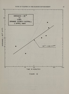
![these experiments. This possibility is substantiated somewhat by considering the data collected on 15 August 1963 near the Redondo Canyon in Santa Monica Bay. On this day the water was particularly clear, but the average stability was comparable to values obtained within the waste field at Orange County. Vertical diffu- sion was suppressed as indicated by the empirical equation for the diffusion parameter o?, (Table 5). However, the value of M’ (78 percent) compares favor- ably with those determined within the waste field. It appears that on days of relatively low stability which results in an increase in vertical diffusion (see next section), the sampling technique may be less accurate. Whatever the reason for the discrepancy in the cal- culated values of M’ within and outside the waste field, it appears that it was not the result of photochemical decay, water temperature fluctuations, or physical adsorption. All experiments were conducted at or very near the water surface, where photochemical and tem- perature effects presumably would be similar regardless of the location of the test area. Physical adsorption, if appreciable, probably would occur more readily within the waste field where the concentrations of organic solids were higher than at the background sites. If any- thing, lower values of M’ would be expected for ex- periments conducted within the waste field but just the reverse was true in these experiments. 8. EFFECTS OF WIND AND STABILITY ON DIFFUSION PARAMETERS One of the principal objectives of this research has been to demonstrate, if possible, the effect of water column stability and wind speed on the rate of vertical eddy diffusion. For the case of relative diffusion at the surface of the ocean, it has often been speculated (16) that the presence of a strong positive density gradient with depth (a highly stable water column) can only result in a supression of vertical turbulence and a con- comittant decrease in the rate of vertical eddy diffusion. This speculation has been confirmed somewhat by Kellogg (17) whose investigations on the diffusion of smoke puffs in the atmosphere showed that a decrease in the mass rate of puff growth occurred with increasing atmospheric stability. On the basis of Kellogg’s work it was believed a similar effect could be demonstrated in the ocean. To the oceanographer the term “stability” generally refers to the definition presented by Sverdrup et al. (16): Op es tool tas0P Ee ee AZ ned (11) where p is the density of sea water defined by ps,6,p that is, p is the density zn sctu at a salinity s, a tempera- ture @ and a pressure p. A distinction is usually made between the density in situ and that at atmospheric pressure, ps,e,o. The difference between the two is due to the compressibility of water at the particular tem- perature and salinity. When working in relatively shallow depths the difference may be neglected. In order to avoid writing a large number of decimals, the density (ps,6,0) is normally expressed by the symbol sigma-t, defined by: An approximate form of (11), accurate within the first 300 feet of the water surface, is expressed as: , _ dor ag = dz Pat (13) Where Z is the depth in meters. Actually E’ is the slope of the o; curve in relation to depth and can be positive, neutral, or negative. A water column is classified as stable, indifferent, or unstable depending on the sign of EK’. In these experiments stability has been arbi- trarily defined, for reasons of convenience, as S’ = EB’ Xx 10? The importance of selecting the proper depth interval when computing and interpreting values of S’ within a waste field has been discussed by Gunnerson (18). Early experiments conducted around the Orange County outfall indicated that at 50 to 100 feet from the axis of the boil the depth of the field was less than 3 meters. Consequently, temperature and salinity data for sta- bility computations were collected at 0, 3, 6 and 12 meter depths. Stability data for the 0-3 meter interval were found to give the strongest correlation with mea- surements of vertical diffusion and all values of S’ used in this report therefore are for this depth interval. Stability within the waste field was highly variable. S’ ranged from highly positive values of 500 to 5800 near the boil, to low positive and sometimes negative values at 200 to 250 minutes after dye release. Figure 17 is a semi-log plot of the observed values of 8’ de- termined on 11 April 1963. It is evident that the sta- bility decreases quite rapidly from an initial high positive value at the boil to values of S’ approaching that of the background water at around 300 minutes downstream. Data collected during two experiments off Catalina Island are also shown for comparison in Figure 17. On these days the stability also varied with time, probably due to heating of the surface layers, but the individual values of S’ were considerably lower than corresponding values observed within the waste field. The space-time variation of 8’ within the field is the result of further dilution of the effluent mixture with adjacent and underlying water masses. As the field di- lutes with time, the surface salinity increases, thus decreasing observed values of S’. The same space-time variation has been observed with respect to inorganic nutrient and tracer dye concentrations as shown in Figure 18. Because of this pronounced time variation of stability within the field, it is necessary to use a time-averaging process to arrive at comparable values of S’. The average stability at any time is defined as ae Yi) .-194 (2S) aT + tie] wad aa Sieg 2 where S’ is the average stability at time T minutes after dye discharge. For experiments where no boil samples were taken, the average of all observed boil stabilities (4500) was arbitrarily used. The computed average values of S’ for all experiments at or about 200 minutes after dye](https://iiif.wellcomecollection.org/image/b32172370_0042.jp2/full/800%2C/0/default.jpg)